1 Introduction and data sets
In the book, examples of event history data are used to illustrate different methods, models and approaches. All the data sets, except the LEADER data, are available for download as CSV files and description of the variables is given below.
1.1 PBC3 trial in liver cirrhosis
| Variable name | Description |
|---|---|
id |
patient id |
unit |
hospital |
days |
follow-up time in days |
status |
0 = censoring, 1 = transplantation, 2 = death without transplantation |
tment |
randomized treatment: 0 = placebo, 1 = CyA |
sex |
0 = female, 1 = male |
age |
age in years |
bili |
bilirubin (micromoles/L) |
alb |
albumin (g/L) |
stage |
disease stage: 2 = I-II, 3 = III, 4 = IV |
Read data and in-text summary
Code show/hide
pbc3 <- read.csv("data/pbc3.csv")
pbc3$fail <- ifelse(pbc3$status != 0, 1, 0) # event/failure indicator
pbc3$tment_char <- ifelse(pbc3$tment == 0, "Placebo", "CyA")
addmargins(table(pbc3$status,pbc3$tment_char))
      CyA Placebo Sum
  0   132     127 259
  1    14      15  29
  2    30      31  61
  Sum 176     173 349
Code show/hide
proc import out=pbc3
    datafile="data/pbc3.csv"
    dbms=csv replace;
run;
proc freq data=pbc3;
  table status*tment;
run;
1.2 Guinea-Bissau childhood vaccination study
| Variable name | Description |
|---|---|
id |
child id |
cluster |
cluster id |
fuptime |
follow-up time (days) |
dead |
0 = alive, 1 = dead |
bcg |
bcg vaccination status at initial visit: 0 = no, 1 = yes |
dtp |
no of dtp vaccinations at initial visit |
sex |
0 = female, 1 = male |
age |
age in days at initial visit |
Read data and Table 1.1
Code show/hide
bissau <- read.csv("data/bissau.csv")
bissau$vaccine <- 1*(bissau$bcg==1 | bissau$dtp>0)
# Table 1.1

addmargins(table(bissau$vaccine,bissau$dead))
         0    1  Sum
  0   1847   95 1942
  1   3205  127 3332
  Sum 5052  222 5274
Code show/hide
with(bissau, table(vaccine, dead)) / rowSums(with(bissau, table(vaccine, dead))) dead
vaccine 0 1
0 0.95108136 0.04891864
1 0.96188475 0.03811525or
Code show/hide
library(procs)
proc_freq(bissau, tables = vaccine*dead, output = report)
CAT Statistic 0 1 Total
1 0 Frequency 1847.00000 95.000000 1942.00000
2 0 Percent 35.02086 1.801289 36.82215
3 0 Row Pct 95.10814 4.891864 NA
4 0 Col Pct 36.55978 42.792793 NA
5 1 Frequency 3205.00000 127.000000 3332.00000
6 1 Percent 60.76981 2.408039 63.17785
7 1 Row Pct 96.18848 3.811525 NA
8 1 Col Pct 63.44022 57.207207 NA
9 Total Frequency 5052.00000 222.000000 5274.00000
10 Total Percent 95.79067 4.209329 100.00000Code show/hide
proc import out=bissau
    datafile="data/bissau.csv"
    dbms=csv replace;
run;
data bissau;
    set bissau;
    vaccine= bcg=1 or dtp>0;
run;
proc freq data=bissau;
    table vaccine*dead;
run;
1.3 Testis cancer incidence and maternal parity
| Variable name | Description |
|---|---|
age |
age of son |
| 0 = 0-14 years | |
| 15 = 15-19 years | |
| 20 = 20-24 years | |
| 25 = 25-29 years | |
| 30 = 30+ years | |
pyrs |
person years at risk |
cases |
number of testis cancer cases |
semi |
number of seminoma cases |
nonsemi |
number of non-seminoma cases |
parity |
parity of mother at birth of son |
cohort |
son cohort (year of birth) |
| 1950 = 1950-1957 | |
| 1958 = 1958-1962 | |
| 1963 = 1963-1967 | |
| 1968 = 1968-1972 | |
| 1973 = 1973-1992 | |
motherage |
mother’s age at birth of son |
| 12 = 12-19 | |
| 20 = 20-24 | |
| 25 = 25-29 | |
| 30 = 30+ |
Read data and in-text summary
Code show/hide
testis <- read.csv("data/testis.csv")
# Add extra variables
testis$lpyrs <- log(testis$pyrs)
testis$par2 <- as.numeric(testis$parity < 2)

library(procs)
proc_means(testis, var = v(pyrs, cases, semi, nonsemi) , stats=v(sum), class=par2)
CLASS TYPE FREQ VAR SUM
1 <NA> 0 237 pyrs 15981967
2 <NA> 0 237 cases 626
3 <NA> 0 237 semi 183
4 <NA> 0 237 nonsemi 443
5 0 1 176 pyrs 8009691
6 0 1 176 cases 228
7 0 1 176 semi 62
8 0 1 176 nonsemi 166
9 1 1 61 pyrs 7972276
10 1 1 61 cases 398
11 1 1 61 semi 121
12 1 1 61 nonsemi 277Code show/hide
proc import out=testis
    datafile="data/testis.csv"
    dbms=csv replace;
run;
data testis;
  set testis;
  par2 = (parity>=2);
run;
proc means data=testis sum;
  var pyrs cases semi nonsemi;
run;
proc means data=testis sum;
  class par2;
  var cases pyrs;
run;
1.4 PROVA trial in liver cirrhosis
| Variable name | Description |
|---|---|
id |
patient id |
timedeath |
followup time (days) |
death |
0 = alive, 1 = dead |
timebleed |
time to bleeding (days); missing if bleed = 0 |
bleed |
0 = no bleeding, 1 = bleeding |
beta |
0 = no propranolol, 1 = propranolol |
scle |
0 = no sclerotherapy, 1 = sclerotherapy |
sex |
0 = female, 1 = male |
age |
age (years) |
bili |
bilirubin (micromoles/L) |
coag |
coagulation factors (% of normal) |
varsize |
variceal size: 1 = small, 2 = medium, 3 = large |
Read data and Table 1.2
Code show/hide
prova <- read.csv("data/prova.csv", na.strings = c("."))
# Treatment 2x2 factorial
prova$beh <- with(prova, as.factor(scle + beta*2))
# 0 = none
# 1 = sclerotherapy only
# 2 = propranolol only
# 3 = both
with(prova, table(beh))
beh
0 1 2 3
72 73 68 73 Code show/hide
# Bleeding
with(prova, table(beh, bleed))
bleed
beh 0 1
0 59 13
1 60 13
2 56 12
3 61 12Code show/hide
# Death
with(prova, table(beh, death))
death
beh 0 1
0 56 16
1 55 18
2 57 11
3 43 30Code show/hide
# Death w/o bleed
with(subset(prova, bleed == 0), table(beh, death))
death
beh 0 1
0 51 8
1 47 13
2 51 5
3 41 20Code show/hide
# Death after bleed
with(subset(prova, bleed == 1), table(beh, death))
death
beh 0 1
0 5 8
1 8 5
2 6 6
3 2 10Code show/hide
proc import out=prova
    datafile="data/prova.csv"
    dbms=csv replace;
run;
data prova;
    set prova;
    beh = scle + beta*2;
run;
/*
0 = none
1 = sclerotherapy only
2 = propranolol only
3 = both
*/
proc freq data=prova;
    table beh beh*bleed beh*death bleed*beh*death;
run;
1.5 Recurrent episodes in affective disorders
Note, that all patients start in state 1 (in hospital).
| Variable name | Description |
|---|---|
id |
patient id |
episode |
number of affective episodes |
state |
Status at time start: |
| 0 = no current affective episode, 1 = current affective episode | |
start |
start time in state (months) |
stop |
last time seen in state (months) |
status |
status at time stop: |
| 0 = transition to state 0 | |
| 1 = transition to state 1 | |
| 2 = transition to death | |
| 3 = censoring | |
bip |
0 = unipolar, 1 = bipolar |
sex |
0 = female, 1 = male |
age |
age (years) |
year |
year of initial episode |
Read data and in-text summary
Code show/hide
affective <- read.csv("data/affective.csv")
length(unique(affective$id))
[1] 119Code show/hide
length(unique(affective$id[affective$bip==0]))[1] 98Code show/hide
length(unique(affective$id[affective$bip==1]))[1] 21Code show/hide
# The patients starts in state 1 (at hospital)
(sum(affective$status==1)+length(unique(affective$id)))/length(unique(affective$id))
[1] 5.554622Code show/hide
table(affective$status)
  0   1   2   3
626 542  78  41
Code show/hide
proc import out=affective
    datafile="data/affective.csv"
    dbms=csv replace;
run;
proc sql;
  select bip, count(distinct id) as n
  from affective
    group by bip;
quit;
proc freq data=affective;
  table status;
run;
1.6 LEADER cardiovascular trial in type 2 diabetes
Data not available for download.
Two data sets are used in the code:
Recurrent MI: leader_mi
Recurrent myocardial infarction (MI) with all-cause death as competing risk.
| Variable name | Description |
|---|---|
id |
patient id |
start |
start time to event (days since randomization) |
stop |
stop time (days since randomization) |
status |
status at stop: |
| 0 = censoring | |
| 1 = recurrent myocardial infarction | |
| 2 = all cause death | |
eventno |
event number (1, 2, 3, …) |
treat |
randomized treatment: 0 = placebo, 1 = liraglutide |
Recurrent 3-p MACE: leader_3p
Recurrent events of a 3-point MACE (major adverse cardiovascular events) consisting of non-fatal myocardial infarction, non-fatal stroke, or cardiovascular death.
| Variable name | Description |
|---|---|
id |
patient id |
start |
start time to event (days since randomization) |
stop |
stop time (days since randomization) |
status |
status at stop: |
| 0 = censoring | |
| 1 = recurrent myocardial infarction | |
| 2 = recurrent stroke | |
| 3 = cardiovascular death | |
| 4 = non-cardiovascular death | |
eventno |
event number (1, 2, 3, …) |
treat |
randomized treatment: 0 = placebo, 1 = liraglutide |
Read data and Table 1.3
Assume that the LEADER data sets are loaded.
Code show/hide
# For recurrent MI
length(unique(leader_mi$id)) # n randomized
[1] 9340Code show/hide
with(subset(leader_mi,treat==1), length(unique(id))) # n for liraglutide[1] 4668Code show/hide
with(subset(leader_mi,treat==0), length(unique(id))) # n for placebo[1] 4672Code show/hide
with(subset(leader_mi, eventno==1), table(status, treat)) # >=1 event and dead/censored before 1st event treat
status 0 1
0 3960 4047
1 339 292
2 373 329Code show/hide
with(subset(leader_mi, status==1), table(treat)) # Total eventstreat
0 1
421 359 Code show/hide
# For recurrent 3p MACE
length(unique(leader_3p$id)) # n randomized
[1] 9340Code show/hide
with(subset(leader_3p,treat==1), length(unique(id))) # n for liraglutide[1] 4668Code show/hide
with(subset(leader_3p,treat==0), length(unique(id))) # n for placebo[1] 4672Code show/hide
with(subset(leader_3p, eventno==1), table(status, treat)) # >=1 event and dead/censored before 1st event treat
status 0 1
0 3845 3923
1 325 286
2 181 163
3 188 159
4 133 137Code show/hide
with(subset(leader_3p, status==1), table(treat)) # Total eventstreat
0 1
421 359 Code show/hide
* Recurrent MI;
data leader_mi;
    set leader;
    where type = "recurrent_mi";
run;
proc sql;
  select treat, count(distinct id) as n
  from leader_mi
    group by treat
  union
  select . as treat, count(distinct id) as total
  from leader_mi;
quit;

* >=1 event and dead/censored before 1st event;
proc freq data=leader_mi;
  where eventno=1;
    tables status*treat;
run;
* Total events;
proc freq data=leader_mi;
  where status=1;
    tables treat;
run;

* Recurrent 3p-MACE;
data leader_3p;
    set leader;
    where type = "recurrent_comb";
run;
proc sql;
  select treat, count(distinct id) as n
  from leader_3p
    group by treat
  union
  select . as treat, count(distinct id) as total
  from leader_3p;
quit;
* >=1 event and dead/censored before 1st event;
proc freq data=leader_3p;
  where eventno=1;
    tables status*treat;
run;
* Total events;
proc freq data=leader_3p;
  where status=1;
    tables treat;
run;
1.7 Bone marrow transplantation in acute leukemia
| Variable name | Description |
|---|---|
id |
patient id |
team |
team id |
timedeath |
followup time (months) |
death |
0 = alive, 1 = dead |
timerel |
time to relapse (months); missing if rel = 0 |
rel |
0 = no replase, 1 = relapse |
timegvhd |
time to GvHD (months); missing if gvhd = 0 |
gvhd |
0 = no GvHD, 1 = GvHD |
timeanc500 |
time to absolute neutrophil count (ANC) above 500 cells per \(\mu\)L; missing if anc500 = 0 |
anc500 |
0 = ANC below 500, 1 = ANC above 500 |
sex |
0 = female, 1 = male |
age |
age (years) |
all |
0 = acute myelogenous leukemia (AML) |
| 1 = acute lymphoblastic leukemia (ALL) | |
bmonly |
0 = peripheral blood/bone marrow, 1 = only bone marrow |
Read data and Table 1.4
Code show/hide
bmt <- read.csv("data/bmt.csv")

with(bmt, table(rel))
rel
0 1
1750 259 Code show/hide
with(bmt, table(rel)) / sum(with(bmt, table(rel)))rel
0 1
0.8710801 0.1289199 Code show/hide
with(bmt, table(death))death
0 1
1272 737 Code show/hide
with(bmt, table(death)) / sum(with(bmt, table(death)))death
0 1
0.6331508 0.3668492 Code show/hide
with(bmt, table(rel,death)) death
rel 0 1
0 1245 505
1 27 232Code show/hide
with(bmt, table(rel,death)) / rowSums(with(bmt, table(rel,death))) death
rel 0 1
0 0.7114286 0.2885714
1 0.1042471 0.8957529Code show/hide
with(bmt, table(gvhd))gvhd
0 1
1033 976 Code show/hide
with(bmt, table(gvhd)) / sum(with(bmt, table(gvhd)))gvhd
0 1
0.5141862 0.4858138 Code show/hide
with(bmt, table(gvhd, rel)) rel
gvhd 0 1
0 865 168
1 885 91Code show/hide
with(bmt, table(gvhd, rel)) / rowSums(with(bmt, table(gvhd, rel))) rel
gvhd 0 1
0 0.8373669 0.1626331
1 0.9067623 0.0932377Code show/hide
with(bmt, table(gvhd, death)) death
gvhd 0 1
0 685 348
1 587 389Code show/hide
with(bmt, table(gvhd, death)) / rowSums(with(bmt, table(gvhd, death))) death
gvhd 0 1
0 0.6631171 0.3368829
1 0.6014344 0.3985656Code show/hide
proc import out=bmt
    datafile="data/bmt.csv"
    dbms=csv replace;
run;
proc freq data=bmt;
    table rel death rel*death gvhd gvhd*rel gvhd*death;
run;
1.8 The Copenhagen Holter study
| Variable name | Description |
|---|---|
id |
patient id |
timedeath |
followup time (days) |
death |
0 = alive, 1 = dead |
timeafib |
time to atrial fibrillation (days); missing if afib = 0 |
afib |
0 = no atrial fibrillation, 1 = atrial fibrillation |
timestroke |
time to stroke (days); missing if stroke = 0 |
stroke |
0 = no stroke, 1 = stroke |
sex |
0 = female, 1 = male |
age |
age (years) |
smoker |
current smoker: 0 = no, 1 = yes |
esvea |
excessive supra-ventricular ectopic activity: 0 = no, 1 = yes |
chol |
cholesterol (mmol/L) |
diabet |
diabets mellitus: 0 = no, 1 = yes |
bmi |
body mass index (kg/m\(^2\)) |
aspirin |
aspirin use: 0 = no, 1 = yes |
probnp |
NT-proBNP (pmol/L) |
sbp |
systolic blood pressure (mmHg) |
Read data and Table 1.5
Code show/hide
holter <- read.csv("data/cphholter.csv")
with(holter, table(esvea)) # total
esvea
0 1
579 99 Code show/hide
with(holter, table(afib, stroke, death, esvea)), , death = 0, esvea = 0
stroke
afib 0 1
0 320 17
1 29 7
, , death = 1, esvea = 0
stroke
afib 0 1
0 158 25
1 20 3
, , death = 0, esvea = 1
stroke
afib 0 1
0 34 1
1 8 1
, , death = 1, esvea = 1
stroke
afib 0 1
0 32 14
1 4 5Code show/hide
with(subset(holter, timeafib <= timestroke),
     table(afib, stroke, death, esvea)) # 0 -> AF -> Stroke -> dead (yes/no)
, , death = 0, esvea = 0
stroke
afib 1
1 3
, , death = 1, esvea = 0
stroke
afib 1
1 2
, , death = 0, esvea = 1
stroke
afib 1
1 1
, , death = 1, esvea = 1
stroke
afib 1
1 3Code show/hide
with(subset(holter, timestroke < timeafib),
     table(afib, stroke, death, esvea)) # 0 -> Stroke -> AF -> dead (yes/no)
, , death = 0, esvea = 0
stroke
afib 1
1 4
, , death = 1, esvea = 0
stroke
afib 1
1 1
, , death = 0, esvea = 1
stroke
afib 1
1 0
, , death = 1, esvea = 1
stroke
afib 1
1 2Code show/hide
proc import
  datafile="data/cphholter.csv"
    out=holter
    dbms = csv
    replace;
run;

*--- Table 1.5 -------------------------------;

    proc freq data=holter;
  title 'Total';
    tables esvea / nocol norow nopercent;
run;

proc freq data=holter;
    title '';
    tables afib*stroke*death*esvea / nocol norow nopercent;
run;

proc freq data=holter;
    title '0 -> AF -> Stroke -> dead (yes/no)';
    where .<timeafib <= timestroke;
    tables afib*stroke*death*esvea / nocol norow nopercent;
run;

proc freq data=holter;
    title '0 -> Stroke -> AF -> dead (yes/no)';
    where .<timestroke < timeafib;
    tables afib*stroke*death*esvea / nocol norow nopercent;
run;
1.9 Small set of survival data
Only done in R.
Create data
Code show/hide
times <- c(5,6,7,8,9,12,13,15,16,20,22,23)
age <- c(12,0,0,10,6,6,9,3,8,0,0,2)
event <- c(1,0,1,1,0,0,1,1,1,0,0,1)
id <- 1:12
exitage <- age + times
simpledata <- as.data.frame(cbind(id, times, event, age, exitage))
Figure 1.8
Code show/hide
#------------------------------------------------------------------#
# General plotting styles
#------------------------------------------------------------------#
library(ggplot2)
theme_general <- theme_bw() +
  theme(legend.position = "none",
        text = element_text(size = 20),
        axis.text.x = element_text(size = 20),
        axis.text.y = element_text(size = 20))

theme_general_x <- theme_bw() +
  theme(legend.position = "none",
        text = element_text(size = 26),
        axis.text.x = element_text(size = 26),
        axis.text.y = element_text(size = 26))

# Create Figure 1.8, part (a)
fig1.8a <- ggplot(aes(x = times, y = id), data = simpledata) +
  geom_segment(aes(x = 0, y = id, xend = times - 0.25, yend = id), size = 1) +
  geom_point(aes(x = times, y = id), data = subset(simpledata,event==0),
             shape = 21, size = 6, color='black', fill='white') +
  geom_point(aes(x = times, y = id), data = subset(simpledata,event==1),
             shape = 16, size = 6) +
  xlab("Time (t)") +
  ylab("Subject number") +
  scale_x_continuous(expand = expansion(mult = c(0.005, 0.05)),
                     limits = c(0, 25)) +
  scale_y_continuous(expand = expansion(mult = c(0.005, 0.05)),
                     limits = c(0.5, 12), breaks = seq(1, 12, 1)) +
  theme_general_x +
  theme(panel.grid.major.y = element_blank(),
        panel.grid.minor.y = element_blank())

fig1.8a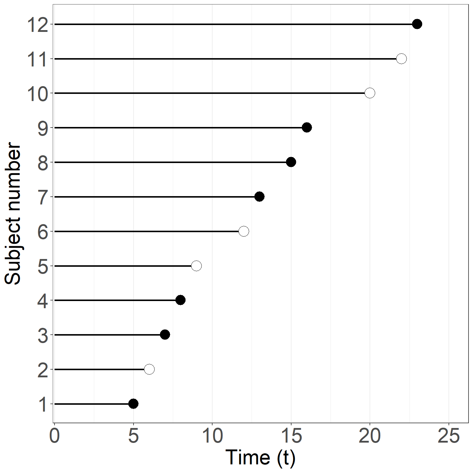
Code show/hide
# Create Figure 1.8, part (b)
fig1.8b <- ggplot(aes(x = exitage, y = id), data = simpledata) +
  geom_segment(aes(x = age, y = id, xend = exitage - 0.25, yend = id), size = 1) +
  geom_point(aes(x = exitage, y = id), data = subset(simpledata,event==0),
             shape = 21, size = 6, color='black', fill='white') +
  geom_point(aes(x = exitage, y = id), data = subset(simpledata,event==1),
             shape = 16, size = 6) +
  xlab("Age") +
  ylab("Subject number") +
  scale_x_continuous(expand = expansion(mult = c(0.005, 0.05)),
                     limits = c(0, 25)) +
  scale_y_continuous(expand = expansion(mult = c(0.005, 0.05)),
                     limits = c(0.5, 12), breaks = seq(1, 12, 1)) +
  theme_general_x +
  theme(legend.position = "none",
        panel.grid.major.y = element_blank(),
        panel.grid.minor.y = element_blank())

fig1.8b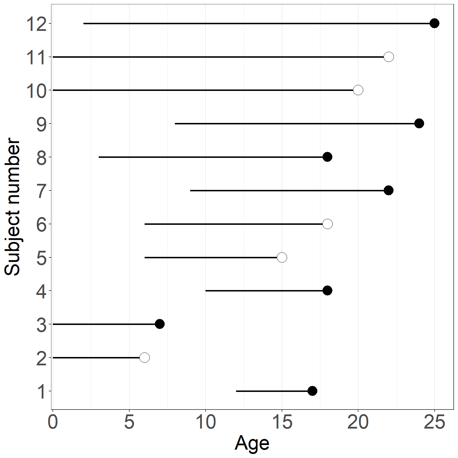
Figure 1.9
Code show/hide
#------------------------------------------------------------------#
# Figure 1.9
#------------------------------------------------------------------#
library(survival)
# Kaplan-Meier time as time variable
kmfit <- survfit(Surv(times, event) ~ 1)
simpledata_km <- data.frame(surv = c(1, kmfit$surv),
                            time = c(0, kmfit$time))

# Create Figure 1.9, part (a)
fig1.9a <- ggplot(aes(x = time, y = surv), data = simpledata_km) +
  geom_step(size = 1) +
  xlab("Time (t)") +
  ylab("Estimate of S(t)") +
  scale_x_continuous(expand = expansion(mult = c(0.05, 0.05)),
                     limits = c(0, 25)) +
  scale_y_continuous(expand = expansion(mult = c(0.05, 0.05)),
                     limits = c(0, 1), breaks = seq(0, 1, 0.1)) +
  theme_general_x

fig1.9a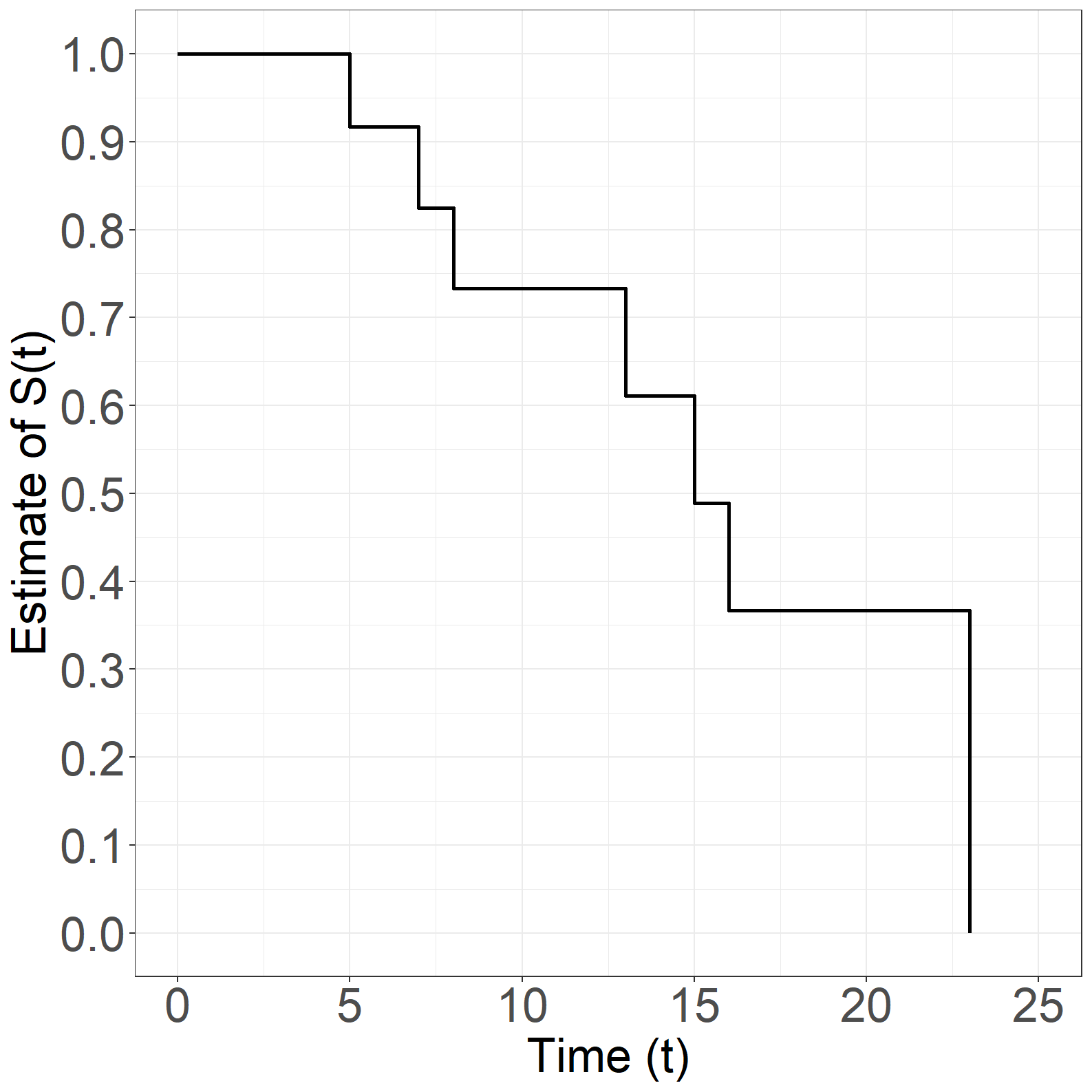
Code show/hide
# Kaplan-Meier age as time variable
kmfit2 <- survfit(Surv(age, exitage, event) ~ 1)
simpledata_km_age <- data.frame(surv = c(1, kmfit2$surv),
                                time = c(0, kmfit2$time))

# Create Figure 1.9, part (b)
fig1.9b <- ggplot(aes(x = time, y = surv), data = simpledata_km_age) +
  geom_step(size = 1) +
  xlab("Age") +
  ylab("Estimate of S(age)") +
  scale_x_continuous(expand = expansion(mult = c(0.05, 0.05)),
                     limits = c(0, 25)) +
  scale_y_continuous(expand = expansion(mult = c(0.05, 0.05)),
                     limits = c(0, 1), breaks = seq(0, 1, 0.1)) +
  theme_general_x

fig1.9b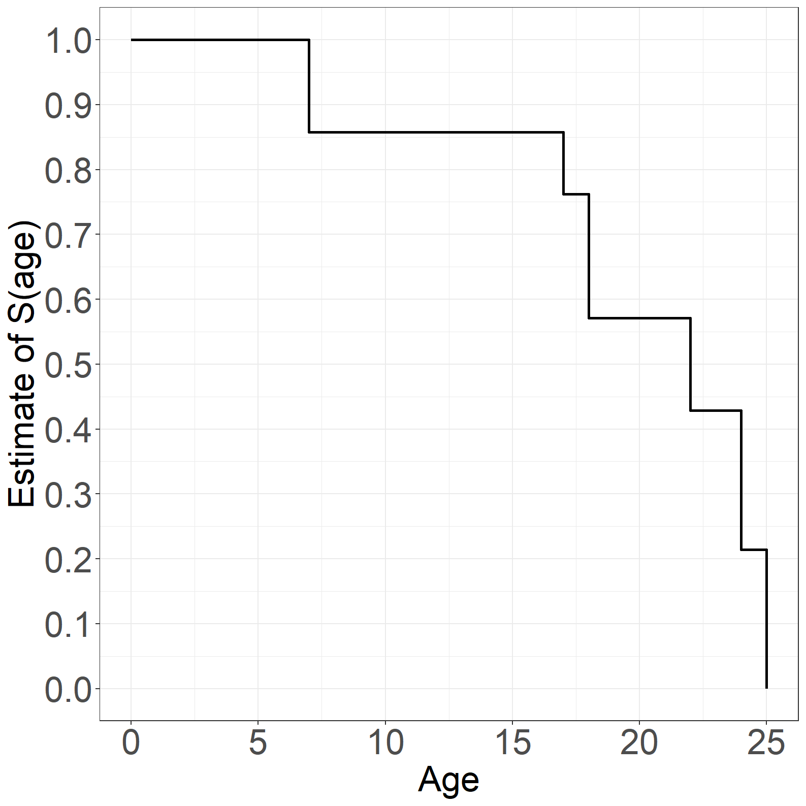
Figure 1.10
Code show/hide
#------------------------------------------------------------------#
# Figure 1.10
#------------------------------------------------------------------#

# Kaplan-Meier time as time variable
kmfit <- survfit(Surv(times, event) ~ 1)
simpledata_km <- data.frame(surv = c(1, kmfit$surv),
                            time = c(0, kmfit$time))
subdata<-simpledata_km[simpledata_km$time<=12,]

# Create Figure 1.10
library(dplyr)
fig1.10 <- ggplot(mapping=aes(x = time, y = surv), data = simpledata_km) +
  geom_rect(data=subdata,
            aes(xmin = time, xmax = lead(time),
                ymin = 0, ymax = surv),
            linetype=0,fill="grey")+
  geom_segment(aes(x = 12, y = -Inf, xend = 12, yend = 0.733),
               size=1,linetype="dashed")+
  geom_step(size = 1) +
  xlab("Time (t)") +
  ylab("Estimate of S(t)") +
  scale_x_continuous(expand = expansion(mult = c(0.05, 0.05)),
                     limits = c(0, 25)) +
  scale_y_continuous(expand = expansion(mult = c(0.05, 0.05)),
                     limits = c(0, 1), breaks = seq(0, 1, 0.1)) +
  theme_general +
  annotate(geom="text",x=6, y=0.45,
           label=expression(epsilon[0](12)),size=8)
fig1.10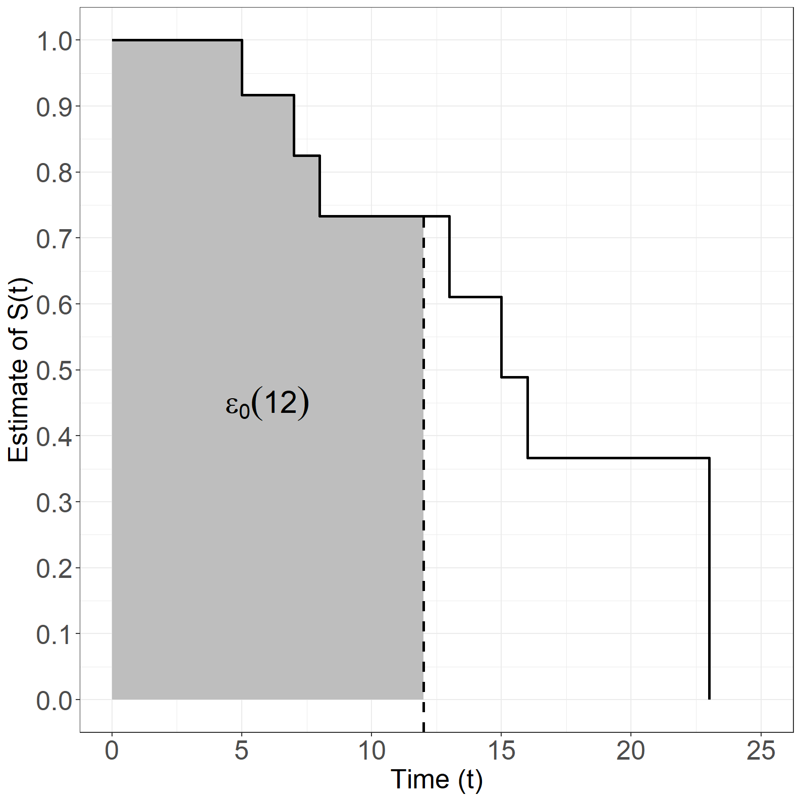
Figure 1.13
Code show/hide
#------------------------------------------------------------------#
# Figure 1.13
#------------------------------------------------------------------#

# N(t)
sfit <- survfit(Surv(times, event) ~ 1)
p1 <- data.frame(time = c(0, sfit$time, 26),
                 n = c(0, cumsum(sfit$n.event), tail(cumsum(sfit$n.event),1)))
p2 <- data.frame(time = sfit$time[sfit$n.event==1],
                 n = cumsum(sfit$n.event)[sfit$n.event==1]-1)
p3 <- data.frame(time = sfit$time[sfit$n.event==1],
                 n = cumsum(sfit$n.event)[sfit$n.event==1])

# Create Figure 1.13, part (a)
fig1.13a <- ggplot(aes(x = time, y = n), data = p1) +
  geom_step(size = 1) +
  geom_point(aes(x = time, y = n), data = p2, shape = 21, size = 6,
             color='black', fill='white') +
  geom_point(aes(x = time, y = n), data = p3, shape = 16, size = 6) +
  xlab("Time (t)") +
  ylab("N(t)") +
  scale_x_continuous(expand = expansion(mult = c(0.005, 0.005)),
                     limits = c(0, 26)) +
  scale_y_continuous(expand = expansion(mult = c(0.05, 0.05)),
                     limits = c(0, 12), breaks = seq(0, 12, 1)) +
  theme_general_x

fig1.13a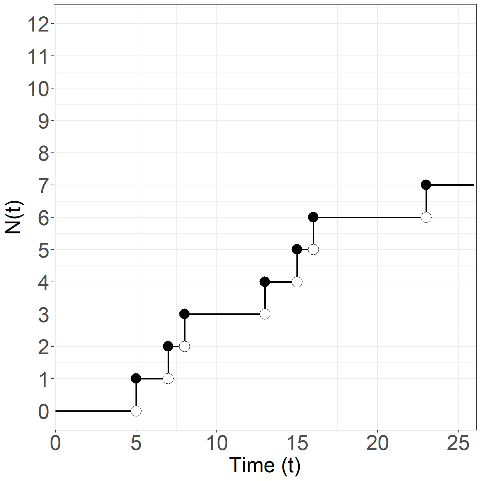
Code show/hide
# Y(t)
sfit <- survfit(Surv(times, event) ~ 1)
p1 <- data.frame(time = c(0, sfit$time, 26),
                 risk = c(sfit$n.risk, 0, 0))
p2 <- data.frame(time = sfit$time,
                 risk = sfit$n.risk - 1)
p3 <- data.frame(time = sfit$time,
                 risk = sfit$n.risk)

# Create Figure 1.13, part (b)
fig1.13b <- ggplot(aes(x = time, y = risk), data = p1) +
  geom_step(size = 1) +
  geom_point(aes(x = time, y = risk), data = p2, shape = 21, size = 6,
             color='black', fill='white') +
  geom_point(aes(x = time, y = risk), data = p3, shape = 16, size = 6) +
  xlab("Time (t)") +
  ylab("Y(t)") +
  scale_x_continuous(expand = expansion(mult = c(0.005, 0.005)),
                     limits = c(0, 26)) +
  scale_y_continuous(expand = expansion(mult = c(0.05, 0.05)),
                     limits = c(0, 12), breaks = seq(0, 12, 1)) +
  theme_general_x

fig1.13b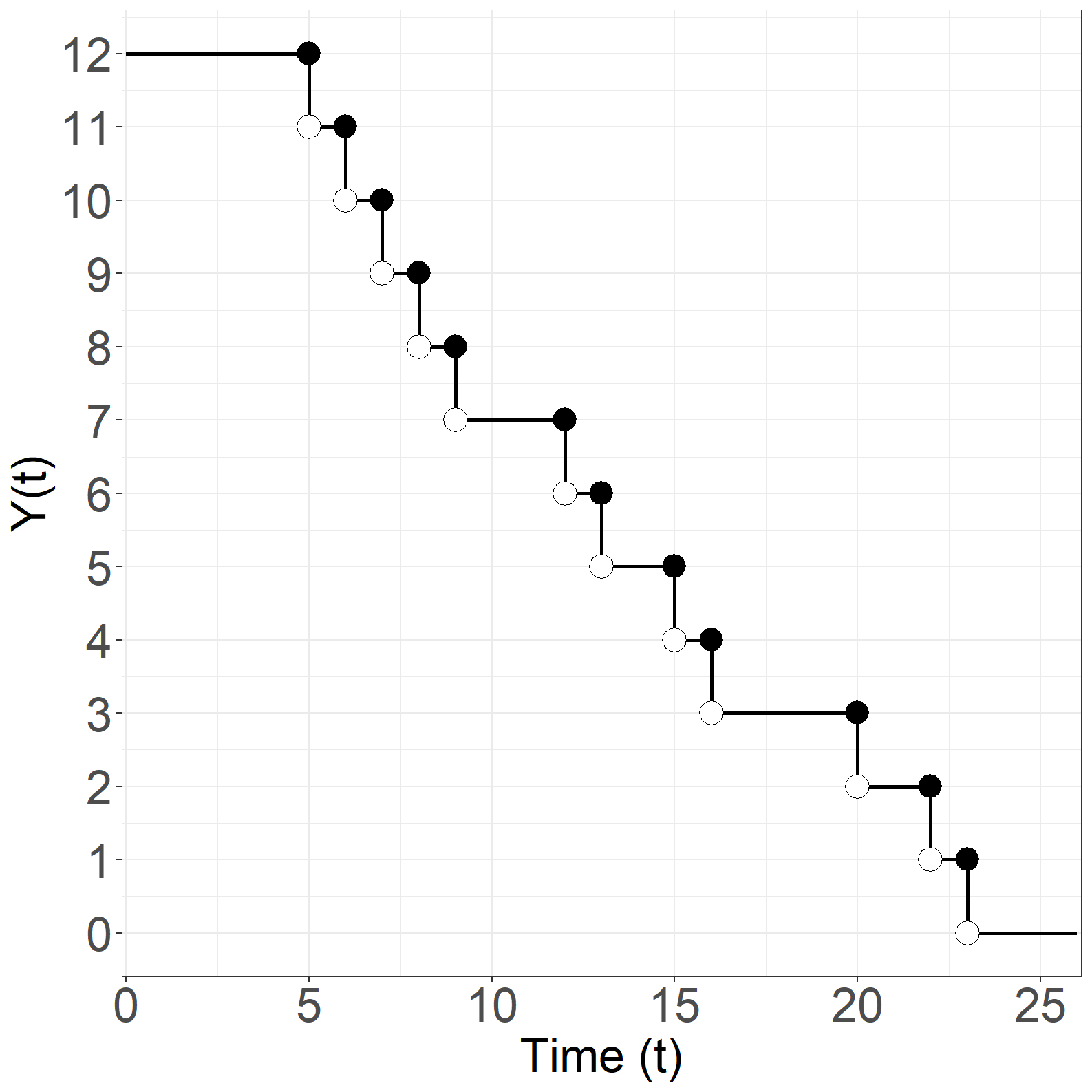
Code show/hide
# N(age)
asfit <- survfit(Surv(age, exitage, event) ~ 1)
p1 <- data.frame(time = c(0, asfit$time, 26),
                 n = c(0, cumsum(asfit$n.event),tail(cumsum(asfit$n.event), 1)))
p2 <- data.frame(time = asfit$time[asfit$n.event > 0],
                 n = cumsum(asfit$n.event)[asfit$n.event > 0])
p3 <- data.frame(time = asfit$time[asfit$n.event > 0],
                 n = c(0, 1, 2, 4, 5, 6))

# Create Figure 1.13, part (c)
fig1.13c <- ggplot(aes(x = time, y = n), data = p1) +
  geom_step(size = 1) +
  geom_point(aes(x = time, y = n), data = p2, shape = 16, size = 6) +
  geom_point(aes(x = time, y = n), data = p3, shape = 21, size = 6,
             color='black', fill='white') +
  xlab("Age") +
  ylab("N(age)") +
  scale_x_continuous(expand = expansion(mult = c(0.005, 0.005)),
                     limits = c(0, 26)) +
  scale_y_continuous(expand = expansion(mult = c(0.05, 0.05)),
                     limits = c(0, 12), breaks = seq(0, 12, 1)) +
  theme_general_x

fig1.13c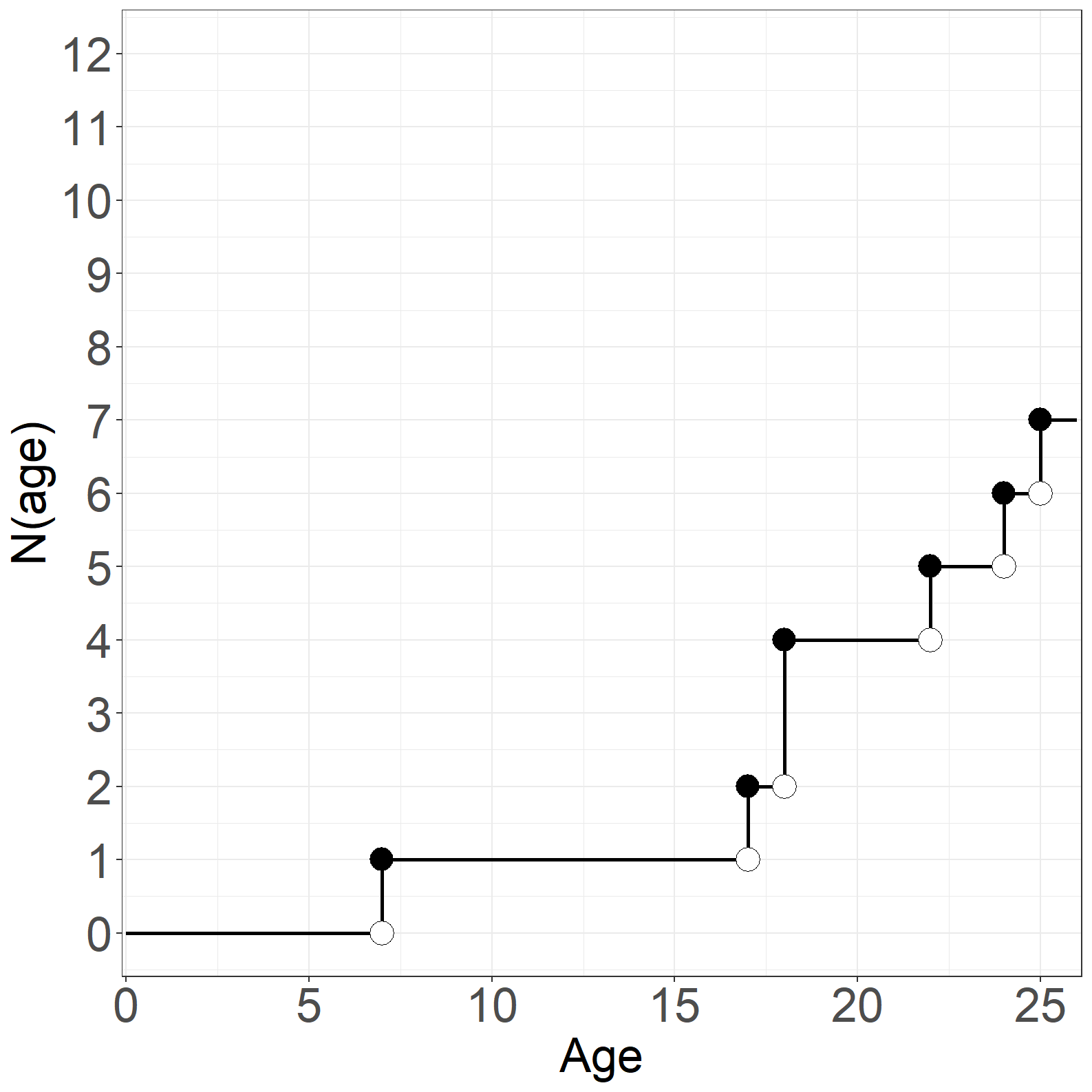
Code show/hide
# Y(age)
atriskage <- vector(length=25)
for(i in 1:25){
  atriskage[i] <- sum((age<=i & exitage>i))
}

p1 <- data.frame(time = 0:26,
                 risk = c(atriskage[1], atriskage, 0))
p2 <- data.frame(time = c(2,3,6,7,8,9,10,12,15,17,18,20,22,24,25),
                 risk = c(5,6,7,6,7,8, 9,10, 9, 8, 5, 4, 2, 1,0))
p3 <- data.frame(time = c(2,3,6,7,8,9,10,12,15,17,18,20,22,24,25),
                 risk = c(4,5,6,7,6,7, 8,9, 10, 9, 8, 5, 4, 2,1))

# Create Figure 1.13, part (d)
fig1.13d <- ggplot(aes(x = time, y = risk), data = p1) +
  geom_step(size = 1) +
  geom_point(aes(x = time, y = risk), data = p2, shape = 21, size = 6,
             color='black', fill='white') +
  geom_point(aes(x = time, y = risk), data = p3, shape = 16, size = 6) +
  xlab("Age") +
  ylab("Y(age)") +
  scale_x_continuous(expand = expansion(mult = c(0.005, 0.005)),
                     limits = c(0, 26)) +
  scale_y_continuous(expand = expansion(mult = c(0.05, 0.05)),
                     limits = c(0, 12), breaks = seq(0, 12, 1)) +
  theme_general_x

fig1.13d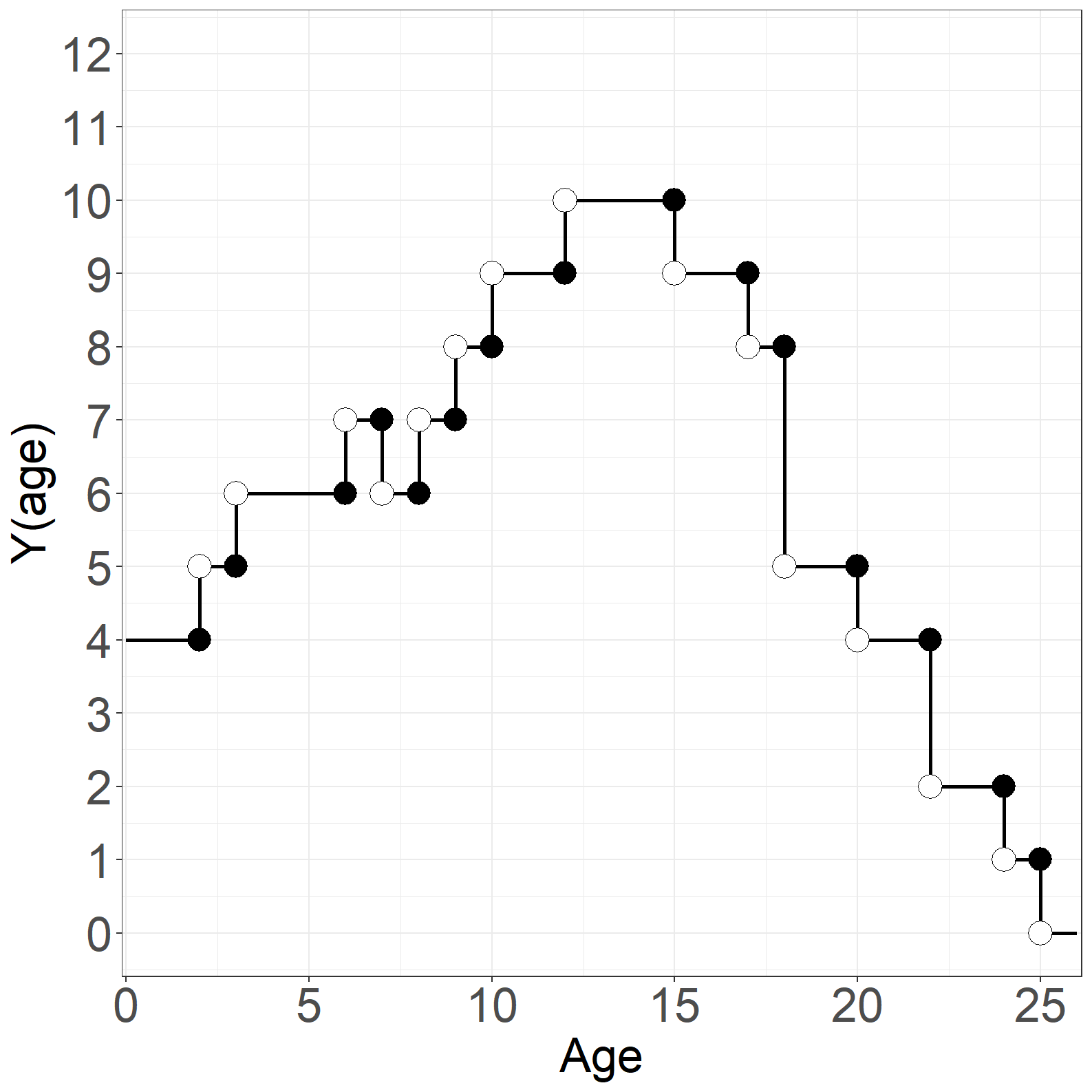
Exercises
The SAS solution is available as a single file for download:
Exercise 1.1
Consider the small data set in Table 1.6 and argue why both the average of all (12) observation times and the average of the (7) uncensored times will likely underestimate the true mean survival time from entry into the study.
The average of all 12 observation times: \[\frac{5+6+7+8+9+12+13+15+16+20+22+23}{12} = \frac{156}{12} = 13.00\] will under-estimate the mean survival time because 5 of the terms in the sum, i.e., those corresponding to right-censored observations, are known to be smaller than the true survival times.
The average of the 7 uncensored observations: \[\frac{5+7+8+13+15+16+23}{7}=\frac{87}{7} = 12.43\] is also likely to under-estimate the mean because right-censoring will typically cause the longer survival times in the population to be incompletely observed. E.g., survival times longer than the time elapsed from the beginning of the study to its end will always be right-censored.
Exercise 1.2
1.
Consider the following records mimicking the Copenhagen Holter study (Example 1.1.8) in wide format and transform them into long format, i.e., create one data set for each of the possible six transitions in Figure 1.7.
Data can (partly) be converted to long format using the msprep function from the mstate package. However, we must first add indicators of whether the subjects transitioned to AF, stroke and death during the study. Furthermore, we have to fill in timeafib, timestroke and timedeath for all subjects, such that they correspond to the last time where transitions to the states AF, stroke and death are possible. Lastly, we need to specify a transition matrix.
Code show/hide
library(tidyverse)
library(survival)
library(mstate)
Code show/hide
# The table from the exercise
id <- factor(1:8)
timeafib <- c(NA, 10, NA, 15, NA, 30, NA, 25)
timestroke <- c(NA, NA, 20, 30, NA, NA, 35, 50)
timedeath <- c(NA, NA, NA, NA, 70, 75, 95, 65)
lastobs <- c(100, 90, 80, 85, 70, 75, 95, 65)
cbind(id, timeafib, timestroke, timedeath, lastobs)
id timeafib timestroke timedeath lastobs
[1,] 1 NA NA NA 100
[2,] 2 10 NA NA 90
[3,] 3 NA 20 NA 80
[4,] 4 15 30 NA 85
[5,] 5 NA NA 70 70
[6,] 6 30 NA 75 75
[7,] 7 NA 35 95 95
[8,] 8 25 50 65 65Code show/hide
# Creating status indicators
afib <- ifelse(is.na(timeafib), 0, 1)
stroke <- ifelse(is.na(timestroke), 0, 1)
death <- ifelse(is.na(timedeath), 0, 1)

# Last time point at risk for a transition to each state
timedeath <- lastobs
timestroke <- ifelse(is.na(timestroke), timedeath, timestroke)
timeafib <- ifelse(is.na(timeafib), timestroke, timeafib)
wide_data <- as.data.frame(cbind(id, timeafib, timestroke,
                                 timedeath, afib, stroke, death))

# Creating the transition matrix without the Stroke to AF transition
tmat <- matrix(NA,4,4)
tmat[1, 2:4] <- 1:3
tmat[2, 3:4] <- 4:5
tmat[3, 4] <- 6
dimnames(tmat) <- list(from = c("No event", "AF", "Stroke", "Death"),
                       to = c("No event", "AF", "Stroke", "Death"))
tmat
to
from No event AF Stroke Death
No event NA 1 2 3
AF NA NA 4 5
Stroke NA NA NA 6
Death NA NA NA NACode show/hide
# Using msprep to create data in long format
long_data <- msprep(time = c(NA, "timeafib", "timestroke", "timedeath"),
                    status = c(NA, "afib", "stroke", "death"),
                    trans = tmat, data = wide_data)

# Now, the Stroke to AF transition is added manually

stroketoaf<-subset(wide_data,stroke==1)

stroketoaf$from <- 3
stroketoaf$to <- 2
stroketoaf$trans <- 7
stroketoaf$Tstart <- stroketoaf$timestroke
stroketoaf$Tstop <- ifelse(stroketoaf$timeafib>stroketoaf$timestroke,timeafib,timedeath)
stroketoaf$status <- ifelse(stroketoaf$timeafib>stroketoaf$timestroke,1,0)
stroketoaf$time <- stroketoaf$Tstop - stroketoaf$Tstart
stroketoaf_long <- subset(stroketoaf, select = c(id,from,to,trans,Tstart,Tstop,time,status))

# and added to the data set created my msprep

finaldata <- rbind(long_data,stroketoaf_long)
head(finaldata)
An object of class 'msdata'
Data:
id from to trans Tstart Tstop time status
1 1 1 2 1 0 100 100 0
2 1 1 3 2 0 100 100 0
3 1 1 4 3 0 100 100 0
4 2 1 2 1 0 10 10 1
5 2 1 3 2 0 10 10 0
6 2 1 4 3 0 10 10 0Create the data.
Code show/hide
data wide_data;
input id timeafib timestroke timedeath lastobs;
datalines;
1 . . . 100
2 10 . . 90
3 . 20 . 80
4 15 30 . 85
5 . . 70 70
6 30 . 75 75
7 . 35 95 95
8 25 50 65 65
;
To convert the data into long format we must first add indicators of whether the subjects transited to AF, stroke and death during the study. Furthermore, we have to fill in timeafib, timestroke and timedeath for all subjects, such that they correspond to the last time where transitions to AF, stroke and death are possible.
We can now create a long format version of the data, i.e. for each subject all relevant transitions h->j correspond to one row in the data set and where trans: transition h -> j:
Tstart: Time of entry into hTstop: Time last seen in hStatus: Transition to j or not at time Tstop
The seven possible transitions are:
0 -> AF
0 -> Stroke
0 -> Dead
AF -> Stroke
AF -> Dead
Stroke -> Dead
Stroke -> AF
Code show/hide
data wide_data;
    set wide_data;
    * Introducing indicators for transitions and last time at risk in each state.;
    if timedeath = . then do; death = 0; end; else do death = 1; end;
    if death = 0 then timedeath = lastobs;
    if timestroke = . then do; stroke = 0; timestroke = timedeath; end; else do; stroke = 1; end;
    if timeafib = . then do; afib = 0; timeafib = timedeath; end; else do; afib = 1; end;
run;

proc print data = wide_data; run;

data long_data;
    set wide_data;
    * Path: 0;
    if ((afib = 0) and (stroke = 0) and (death = 0)) then do;
    trans = 1; Tstart = 0; Tstop = timedeath; status = 0; output;
    trans = 2; Tstart = 0; Tstop = timedeath; status = 0; output;
    trans = 3; Tstart = 0; Tstop = timedeath; status = 0; output; end;
    * Path: 0 -> AF;
    if ((afib = 1) and (stroke = 0) and (death = 0)) then do;
    trans = 1; Tstart = 0; Tstop = timeafib; status = 1; output;
    trans = 2; Tstart = 0; Tstop = timeafib; status = 0; output;
    trans = 3; Tstart = 0; Tstop = timeafib; status = 0; output;
    trans = 4; Tstart = timeafib; Tstop = timedeath; status = 0; output;
    trans = 5; Tstart = timeafib; Tstop = timedeath; status = 0; output; end;
    * Path: 0 -> Stroke;
    if ((afib = 0) and (stroke = 1) and (death = 0)) then do;
    trans = 1; Tstart = 0; Tstop = timestroke; status = 0; output;
    trans = 2; Tstart = 0; Tstop = timestroke; status = 1; output;
    trans = 3; Tstart = 0; Tstop = timestroke; status = 0; output;
    trans = 6; Tstart = timestroke; Tstop = timedeath; status = 0; output;
    trans = 7; Tstart = timestroke; Tstop = timedeath; status = 0; output; end;
    * Path: 0 -> AF -> Stroke;
    if ((afib = 1) and (stroke = 1) and (death = 0) and (timestroke >= timeafib)) then do;
    trans = 1; Tstart = 0; Tstop = timeafib; status = 1; output;
    trans = 2; Tstart = 0; Tstop = timeafib; status = 0; output;
    trans = 3; Tstart = 0; Tstop = timeafib; status = 0; output;
    trans = 4; Tstart = timeafib; Tstop = timestroke; status = 1; output;
    trans = 5; Tstart = timeafib; Tstop = timestroke; status = 0; output;
    trans = 6; Tstart = timestroke; Tstop = timedeath; status = 0; output;
    trans = 7; Tstart = timestroke; Tstop = timedeath; status = 0; output; end;
    * Path: 0 -> Stroke -> AF;
    if ((afib = 1) and (stroke = 1) and (death = 0) and (timestroke < timeafib)) then do;
    trans = 1; Tstart = 0; Tstop = timestroke; status = 0; output;
    trans = 2; Tstart = 0; Tstop = timestroke; status = 1; output;
    trans = 3; Tstart = 0; Tstop = timestroke; status = 0; output;
    trans = 4; Tstart = timeafib; Tstop = timedeath; status = 0; output;
    trans = 5; Tstart = timeafib; Tstop = timedeath; status = 0; output;
    trans = 6; Tstart = timestroke; Tstop = timeafib; status = 0; output;
    trans = 7; Tstart = timestroke; Tstop = timeafib; status = 1; output; end;
    * Path: 0 -> Dead;
    if ((afib = 0) and (stroke = 0) and (death = 1)) then do;
    trans = 1; Tstart = 0; Tstop = timedeath; status = 0; output;
    trans = 2; Tstart = 0; Tstop = timedeath; status = 0; output;
    trans = 3; Tstart = 0; Tstop = timedeath; status = 1; output; end;
    * Path: 0 -> AF -> Dead;
    if ((afib = 1) and (stroke = 0) and (death = 1)) then do;
    trans = 1; Tstart = 0; Tstop = timeafib; status = 1; output;
    trans = 2; Tstart = 0; Tstop = timeafib; status = 0; output;
    trans = 3; Tstart = 0; Tstop = timeafib; status = 0; output;
    trans = 4; Tstart = timeafib; Tstop = timedeath; status = 0; output;
    trans = 5; Tstart = timeafib; Tstop = timedeath; status = 1; output; end;
    * Path: 0 -> Stroke -> Death;
    if ((afib = 0) and (stroke = 1) and (death = 1)) then do;
    trans = 1; Tstart = 0; Tstop = timestroke; status = 0; output;
    trans = 2; Tstart = 0; Tstop = timestroke; status = 1; output;
    trans = 3; Tstart = 0; Tstop = timestroke; status = 0; output;
    trans = 6; Tstart = timestroke; Tstop = timedeath; status = 1; output;
    trans = 7; Tstart = timestroke; Tstop = timedeath; status = 0; output; end;
    * Path: 0 -> AF -> Stroke -> Dead;
    if ((afib = 1) and (stroke = 1) and (death = 1) and (timestroke >= timeafib)) then do;
    trans = 1; Tstart = 0; Tstop = timeafib; status = 1; output;
    trans = 2; Tstart = 0; Tstop = timeafib; status = 0; output;
    trans = 3; Tstart = 0; Tstop = timeafib; status = 0; output;
    trans = 4; Tstart = timeafib; Tstop = timestroke; status = 1; output;
    trans = 5; Tstart = timeafib; Tstop = timestroke; status = 0; output;
    trans = 6; Tstart = timestroke; Tstop = timedeath; status = 1; output;
    trans = 7; Tstart = timestroke; Tstop = timedeath; status = 0; output; end;
    * Path: 0 -> Stroke -> AF -> Dead;
    if ((afib = 1) and (stroke = 1) and (death = 1) and (timestroke < timeafib)) then do;
    trans = 1; Tstart = 0; Tstop = timestroke; status = 0; output;
    trans = 2; Tstart = 0; Tstop = timestroke; status = 1; output;
    trans = 3; Tstart = 0; Tstop = timestroke; status = 0; output;
    trans = 4; Tstart = timeafib; Tstop = timedeath; status = 0; output;
    trans = 5; Tstart = timeafib; Tstop = timedeath; status = 1; output;
    trans = 6; Tstart = timestroke; Tstop = timeafib; status = 0; output;
    trans = 7; Tstart = timestroke; Tstop = timeafib; status = 1; output; end;
    keep id trans Tstart Tstop status;
run;

proc print data = long_data; run;
2.
Do the same for the entire data set.
Read the Copenhagen Holter Study data set.
Code show/hide
chs_data <- read.csv("data/cphholter.csv")We can then repeat the procedure for the full data set:
Code show/hide
chs_data$timestroke <- ifelse(is.na(chs_data$timestroke),
                              chs_data$timedeath, chs_data$timestroke)
chs_data$timeafib <- ifelse(is.na(chs_data$timeafib),
                            chs_data$timestroke, chs_data$timeafib)

chs_long <- msprep(time = c(NA, "timeafib", "timestroke", "timedeath"),
                   status = c(NA, "afib", "stroke", "death"),
                   trans = tmat, data = chs_data)

chs_stroketoaf<-subset(chs_data,stroke==1)

chs_stroketoaf$from <- 3
chs_stroketoaf$to <- 2
chs_stroketoaf$trans <- 7
chs_stroketoaf$Tstart <- chs_stroketoaf$timestroke
chs_stroketoaf$Tstop <- ifelse(chs_stroketoaf$timeafib>chs_stroketoaf$timestroke,chs_stroketoaf$timeafib,chs_stroketoaf$timedeath)
chs_stroketoaf$status <- ifelse(chs_stroketoaf$timeafib>chs_stroketoaf$timestroke,1,0)
chs_stroketoaf$time <- chs_stroketoaf$Tstop - chs_stroketoaf$Tstart
chs_stroketoaf_long <- subset(chs_stroketoaf, select = c(id,from,to,trans,Tstart,Tstop,time,status))


chs_finaldata <- rbind(chs_long,chs_stroketoaf_long)
head(chs_finaldata)
An object of class 'msdata'
Data:
id from to trans Tstart Tstop time status
1 1 1 2 1 0 5396 5396 0
2 1 1 3 2 0 5396 5396 0
3 1 1 4 3 0 5396 5396 0
4 2 1 2 1 0 5392 5392 0
5 2 1 3 2 0 5392 5392 0
6 2 1 4 3 0 5392 5392 0NB: We get a warning because 5 subjects have two events on the same day. This will be handled if necessary for further analyses.
We can now repeat the procedure from above to transform the entire Copenhagen Holter Study data set into long format.
Code show/hide
proc import out = chs_data
  datafile = 'data/cphholter.csv'
  dbms= csv replace;
run;

    data chs_long;
    set chs_data;
    if timestroke = . then timestroke = timedeath;
    if timeafib = . then timeafib = timedeath;
    * Path: 0;
    if ((afib = 0) and (stroke = 0) and (death = 0)) then do;
    trans = 1; Tstart = 0; Tstop = timedeath; status = 0; output;
    trans = 2; Tstart = 0; Tstop = timedeath; status = 0; output;
    trans = 3; Tstart = 0; Tstop = timedeath; status = 0; output; end;
    * Path: 0 -> AF;
    if ((afib = 1) and (stroke = 0) and (death = 0)) then do;
    trans = 1; Tstart = 0; Tstop = timeafib; status = 1; output;
    trans = 2; Tstart = 0; Tstop = timeafib; status = 0; output;
    trans = 3; Tstart = 0; Tstop = timeafib; status = 0; output;
    trans = 4; Tstart = timeafib; Tstop = timedeath; status = 0; output;
    trans = 5; Tstart = timeafib; Tstop = timedeath; status = 0; output; end;
    * Path: 0 -> Stroke;
    if ((afib = 0) and (stroke = 1) and (death = 0)) then do;
    trans = 1; Tstart = 0; Tstop = timestroke; status = 0; output;
    trans = 2; Tstart = 0; Tstop = timestroke; status = 1; output;
    trans = 3; Tstart = 0; Tstop = timestroke; status = 0; output;
    trans = 6; Tstart = timestroke; Tstop = timedeath; status = 0; output;
    trans = 7; Tstart = timestroke; Tstop = timedeath; status = 0; output; end;
    * Path: 0 -> AF -> Stroke;
    if ((afib = 1) and (stroke = 1) and (death = 0) and (timestroke >= timeafib)) then do;
    trans = 1; Tstart = 0; Tstop = timeafib; status = 1; output;
    trans = 2; Tstart = 0; Tstop = timeafib; status = 0; output;
    trans = 3; Tstart = 0; Tstop = timeafib; status = 0; output;
    trans = 4; Tstart = timeafib; Tstop = timestroke; status = 1; output;
    trans = 5; Tstart = timeafib; Tstop = timestroke; status = 0; output;
    trans = 6; Tstart = timestroke; Tstop = timedeath; status = 0; output;
    trans = 7; Tstart = timestroke; Tstop = timedeath; status = 0; output; end;
    * Path: 0 -> Stroke -> AF;
    if ((afib = 1) and (stroke = 1) and (death = 0) and (timestroke < timeafib)) then do;
    trans = 1; Tstart = 0; Tstop = timestroke; status = 0; output;
    trans = 2; Tstart = 0; Tstop = timestroke; status = 1; output;
    trans = 3; Tstart = 0; Tstop = timestroke; status = 0; output;
    trans = 4; Tstart = timeafib; Tstop = timedeath; status = 0; output;
    trans = 5; Tstart = timeafib; Tstop = timedeath; status = 0; output;
    trans = 6; Tstart = timestroke; Tstop = timeafib; status = 0; output;
    trans = 7; Tstart = timestroke; Tstop = timeafib; status = 1; output; end;
    * Path: 0 -> Dead;
    if ((afib = 0) and (stroke = 0) and (death = 1)) then do;
    trans = 1; Tstart = 0; Tstop = timedeath; status = 0; output;
    trans = 2; Tstart = 0; Tstop = timedeath; status = 0; output;
    trans = 3; Tstart = 0; Tstop = timedeath; status = 1; output; end;
    * Path: 0 -> AF -> Dead;
    if ((afib = 1) and (stroke = 0) and (death = 1)) then do;
    trans = 1; Tstart = 0; Tstop = timeafib; status = 1; output;
    trans = 2; Tstart = 0; Tstop = timeafib; status = 0; output;
    trans = 3; Tstart = 0; Tstop = timeafib; status = 0; output;
    trans = 4; Tstart = timeafib; Tstop = timedeath; status = 0; output;
    trans = 5; Tstart = timeafib; Tstop = timedeath; status = 1; output; end;
    * Path: 0 -> Stroke -> Death;
    if ((afib = 0) and (stroke = 1) and (death = 1)) then do;
    trans = 1; Tstart = 0; Tstop = timestroke; status = 0; output;
    trans = 2; Tstart = 0; Tstop = timestroke; status = 1; output;
    trans = 3; Tstart = 0; Tstop = timestroke; status = 0; output;
    trans = 6; Tstart = timestroke; Tstop = timedeath; status = 1; output;
    trans = 7; Tstart = timestroke; Tstop = timedeath; status = 0; output; end;
    * Path: 0 -> AF -> Stroke -> Dead;
    if ((afib = 1) and (stroke = 1) and (death = 1) and (timestroke >= timeafib)) then do;
    trans = 1; Tstart = 0; Tstop = timeafib; status = 1; output;
    trans = 2; Tstart = 0; Tstop = timeafib; status = 0; output;
    trans = 3; Tstart = 0; Tstop = timeafib; status = 0; output;
    trans = 4; Tstart = timeafib; Tstop = timestroke; status = 1; output;
    trans = 5; Tstart = timeafib; Tstop = timestroke; status = 0; output;
    trans = 6; Tstart = timestroke; Tstop = timedeath; status = 1; output;
    trans = 7; Tstart = timestroke; Tstop = timedeath; status = 0; output; end;
    * Path: 0 -> Stroke -> AF -> Dead;
    if ((afib = 1) and (stroke = 1) and (death = 1) and (timestroke < timeafib)) then do;
    trans = 1; Tstart = 0; Tstop = timestroke; status = 0; output;
    trans = 2; Tstart = 0; Tstop = timestroke; status = 1; output;
    trans = 3; Tstart = 0; Tstop = timestroke; status = 0; output;
    trans = 4; Tstart = timeafib; Tstop = timedeath; status = 0; output;
    trans = 5; Tstart = timeafib; Tstop = timedeath; status = 1; output;
    trans = 6; Tstart = timestroke; Tstop = timeafib; status = 0; output;
    trans = 7; Tstart = timestroke; Tstop = timeafib; status = 1; output; end;
    keep id trans Tstart Tstop status;
run;

proc print data = chs_long; run;
Exercise 1.3 (*)
1.
Derive Equations (1.2) and (1.3) for, respectively, the survival function in the two-state model (Figure 1.1) and the cumulative incidence function in the competing risks model (Figure 1.2).
The hazard function \[\alpha(t)=\lim_{dt\rightarrow 0}P(T\leq t+dt\mid T>t)/dt\] equals \[\alpha(t)=\frac{f(t)}{S(t)}=\frac{-(d/dt) S(t)}{S(t)}=-(d/dt)\log S(t)\] where \(f(t)\) is the density function for \(T\) and, thereby, \(S(t)=\exp(-\int_0^t\alpha(u)du)\).
The cause \(h\) cumulative incidence is the probability of failing from cause \(h\) during \([0,t]\). This is the integral of the infinitesimal probabilities of failing in \((u,u+du)\) for \(0\leq u\leq t\). The probability of failing in \((u,u+du)\) is, by definition of the cause-\(h\)-specific hazard, equal to \(S(u)\alpha_h(u)du\) and the desired result \[Q_h(t)=\int_0^tS(u)\alpha_h(u)du\] follows.
2.
Show, for the Markov illness-death model (Figure 1.3), that the state occupation probability for state 1 at time \(t\), \(Q_1(t)\), is \[\int_0^t\exp\left(-\int_0^u(\alpha_{01}(x)+\alpha_{02}(x))dx\right)\alpha_{01}(u)\exp\left(-\int_u^t\alpha_{12}(x)dx\right)du.\]
The probability \(P_{11}(u,t)\) of staying in state 1 from time \(u\) to time \(t\) is given by \(\exp(-\int_u^t\alpha_{12}(x)dx)\) and combining this with the argument from the previous question, i.e., that the (infinitesimal) probability \(\exp(-\int_0^u(\alpha_{01}(x)+\alpha_{02}(x))dx)\alpha_{01}(u)du\), of moving from state 0 to state 1 during \((u, u+du)\), the desired result is obtained by integration over \(u\) from 0 to \(t\).
Exercise 1.4 (*)
Argue (intuitively) how the martingale property \(E(M(t)\mid {\cal H}_{s})=M(s)\) follows from \(E(dM(t)\mid {\cal H}_{t-})=0\) (Section 1.4.3).
Because \(M(s)\) is adapted to the history \({\cal H}_s\) we get \[E(M(t)\mid {\cal F}_s)-M(s)=E(M(t)-M(s)\mid {\cal H}_s).\] We write the difference \(M(t)-M(s)\) as the sum of increments \[=E(\int_{(s,t]}dM(u)\mid {\cal H}_s)\] and change the order of integration and expectation \[=\int_{(s,t]}E(dM(u)\mid {\cal H}_s).\] We finally use the `principle of repeated conditioning’ to obtain the desired result of 0 \[=\int_{(s,t]}E(E(dM(u)\mid {\cal H}_{u-})\mid {\cal H}_s)=0.\]